Preface
A Paper A Day Keep the Doctor Away. 今天的文章是:
Hyperprior Induced Unsupervised Disentanglement of Latent Representations. [paper] [codes] (AAAI2019)
本文通过引入principled hierarchical bayes prior,修改VAE种隐编码的先验p(z)=N(z;0,Σ),将先验的方差作为随机变量,让VAE学习方差的分布。该方法的引入使得我们可以通过控制Σ的期望分布形式,学习隐编码的变量之间的关系的模型,而不仅仅是要求相互独立。
Main Contents
ELBO Decomposition
作者将先验p(z)的形式修改,令p(z)的协方差参数也为一个随机变量Σ。整个生成过程就变成:
p(x,z,Σ)=p(x∣z)p(z∣Σ)p(Σ)
并且使用q(z,Σ∣x)近似推断p(z,Σ∣x),则推导ELBO如下:
Epd(x)[DKL(q(x,z∣Σ)∥p(x,z∣Σ))]=Epd(x)[Eqϕ(z,Σ∣x)[logqϕ(z,Σ∣x)−logpθ(z,Σ∣x)]]=Epd(x)[Eqϕ(z,Σ∣x)[logqϕ(z,Σ∣x)−logpθ(x∣Σ,z)+logp(z,Σ)−logpθ(x)]]>=0
得到ELBO的表达式:
Epd(x)[logpθ(x)]≥Epd(x)[Eqϕ(z,Σ∣x)[logpθ(x∣z,Σ)]−DKL(q(z,Σ∣x)∥p(z,Σ))]=ELBO
以上其实就是标准ELBO的分解过程,只是将原来的一个隐变量z变成(z,Σ)。
但是我们针对KL项,继续分解,并且作者定义后验近似推断的过程为:q(z,Σ∣x)=q(z∣x)q(Σ∣z),则有以下的分解:
−Eqd(x)[DKL(q(z,Σ∣x)∥p(z,Σ))]=−Eqd(x)Eqϕ(z,Σ∣x)[logqϕ(z,Σ∣x)−logp(z,Σ)+logq(z,Σ)−logq(z,Σ)]=−Eqϕ(z,Σ,x)[logq(z,Σ)qϕ(z,Σ∣x)+logp(z,Σ)qϕ(z,Σ)]=−Eqϕ(z,x,Σ)[logqϕ(z)qϕ(Σ∣z)qϕ(z∣x)qϕ(Σ∣z)]−Eqϕ(Σ∣z)qϕ(z)[logp(Σ∣z)p(z)qϕ(Σ∣z)qϕ(z)]=Eqϕ(z,x)[logqϕ(z)qϕ(z∣x)]−Eqϕ(Σ∣z)qϕ(z)[logp(Σ∣z)qϕ(Σ∣z)+logp(z)qϕ(z)]=−(index-code MI)I(x;z)−(marginal KL to prior)Eqϕ(z)DKL(qϕ(Σ∣z)∥p(Σ∣z))−(covariance penalty)DKL(qϕ(z)∥p(z))
上式表明引入之后的KL项可以拆分成index-code ML、marignal prior match、covariance penalty三项,整体可以看成原来的ELBO加上新的covariance penaly这一项。
LELBO=LELBOVAE−Eqϕ(z)DKL(qϕ(Σ∣z)∥p(Σ∣z))
Prior Specification and Inference
ELBO分解之后就是指定Encoder和Decoder中的分布形式:
定义先验中的分布为:
p(Σ)=Wp−1(Σ∣Ψ;v)p(z∣Σ)=N(z;0,Σ)p(x∣z)=N(x;f(z),Σ0)
p(x∣z)的定义不变,而p(z∣Σ)需要Σ。
而Σ满足Inverse-Wishart分布,它的参数为p×p大小的半正定矩阵Ψ(Scale)和v>p−1(自由度)(Σ的大小也为p×p)。均值E[Σ]=(v−p−1)−1Ψ,如果期望的z协方差为Σ0,则Ψ应取(v−p−1)Σ0。而且v起到控制统计独立性的作用,v增大,随机采样的协方差就越接近Σ0。
而推断后验的分布定义为:
q(z∣x)=N(z∣u~;Σ~=L~L~T)u~=g1(x)L~=g2(x)
其中L~为Σ~的Cholesky分解矩阵。
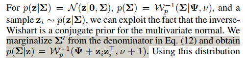
至于q(Σ∣z),作者使用p(Σ∣z)近似估计它:
q(Σ∣z)≈p(Σ∣z)=∫Σ′p(z∣Σ′)p(Σ′)dΣ′p(z∣Σ)p(Σ)
推得:(但是我还并没有理解这里怎么得来的,如下是作者的表述)
图1:近似估计思路
最终得到:
p(Σ∣z)=Wp−1(Ψ+zizi⊤,ν+1)
作者将ELBO继续推导,换了个表述方式(这里的ELBO的表达式和之前的表述不同,从KL项分解的第二个等式继续向下推导):
−Eqϕ(z,Σ,x)[logq(z,Σ)qϕ(z,Σ∣x)+logp(z,Σ)qϕ(z,Σ)]=−Eqϕ(z,Σ,x)[logqϕ(z)qϕ(z∣x)+logp(z∣Σ)p(Σ)qϕ(Σ∣z)qϕ(z)]=−Eqϕ(z,Σ,x)[logp(z∣Σ)qϕ(z∣x)+logp(Σ)qϕ(Σ∣z)]
总体上,ELBO的表达式为:
LELBO=Eq(z∣x)[logp(x∣z)]−Ep(Σ∣z)[DKL(N(μ~,Σ~)∥N(0,Σ))]−Eq(z∣x)[DKL(Wp−1(Φ,λ)∥Wp−1(Ψ,ν))]
这是最终的优化目标。
其他的细节还有:(1)作者使用Bartlett decomposition从inverse-Wishart分布中采样。(2)对使用比较大的v训练模型,作者inference阶段直接使用p(z)=N(z;0,I))采样,也可以生成较好的图像(之前说过v比较大时,各分量趋向于独立)。
以上ELBO的三项的具体计算作者在附录中给出,此处不再赘述。
实验
作者与β-VAE,FactorVAE进行了对比实验,选取FactorVAE提出的metric,在dSprites,CorrelatedEllipses数据集(有groud true factors)上报告了Quantitatiave结果,在3DFaces,3DChairs,CelebA上报告了Qualitative结果。
值得注意的实验结论有:
(1) dSprites上更高的v训练的模型的disentangled效果更好,但是CorrelatedEllipses上,更低的v(v=200)取得了最好的disentangled效果。
(2) 所有模型在捕捉离散的真实factors的表现都不太好。
思维发散
(1) 为什么作者引入Bayes Hyperprior的方法可以更有效地平衡重建误差和Disentangled约束(如作者在第三节开始所述)。也就是,如何思考引入Bayes Hyperpiror的作用?
(2) BF-VAE(Bayes-Factor-VAE)是本文形式的扩展,具体表现在替换了Bayes先验的形式,不是简单地将协方差Σ作为随机变量(因为很可能引起计算上的问题,协方差包含的参数量太大了,O(d*d),d为分量的个数),而是先将p(z)定义成分解的形式,再将各分量的方差组成一个向量,将它作为随机变量(参数量降为O(d)),并且定义的是Gamma分布。